With ACBC, a popular option is to treat the price attribute as a "summed," continuous variable. With summed price, the survey author assigns component-based (level-based) prices (and optionally, a base price for the product). When we display the total price of the product (in the Screener, Choice Tasks, and Calibration sections), we add the prices for its levels (plus any optional base price), and then we vary the price randomly by a user-specified amount of random variation (e.g. -30% to +30%). This has the benefit of displaying overall prices that are more in line with the general quality of the products (for example, it avoids showing a poor product at relatively high prices). But, the drawback is that if price is not varied randomly (and independently) enough, strong enough correlations between price and product features can result and will lead to relatively imprecise estimates of both. In general, we recommend that overall price be varied by at least -30% to +30% to reduce such multicollinearity and ensure reasonably precise estimates. More guidance related to this can be found in the white paper: "Three Ways to Treat Overall Price in Conjoint Analysis" available in our Technical Papers library at www.sawtoothsoftware.com.
Because there are myriad combinations of attribute levels that can make up a product (where each level can have assigned component prices) and prices are varied randomly within a specified range of variation, thousands of unique "displayed" prices can be found across a sample of respondents. To model the effect of price on product choice, we have chosen three effective coding methods: Linear, Log-Linear, and Piecewise.
Linear Function: The total price shown to respondents is coded as a single column in the design matrix. This assumes that the impact of price on utility is a linear effect. (However, note that when projecting respondents' utilities to choices in the simulation module, one typically exponentiates the total utility for products, so the final impact of price on choice probabilities is modestly non-linear.) The benefit of linear coding is that only one parameter is estimated, conserving degrees of freedom. But, if the actual impact of price on utility is non-linear, the linear assumption for this model is simplistic and suboptimal.
(Advanced Note: We temporarily transform whatever price range you provide to the range -1 to +1 for coding in the design matrix so that HB converges quickly. Then, we re-expand the parameters back to the original scale when reporting the final utilities.)
Log-Linear Function: The total price shown to respondents is transformed by the natural log and coded as a single column in the design matrix. This assumes that the impact of price on utility is log-linear, or somewhat curved, as shown below:
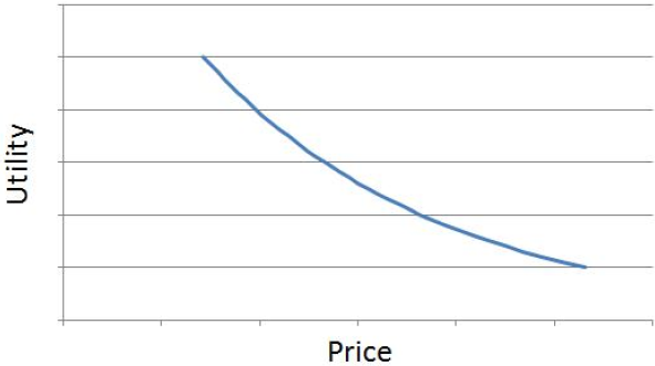
As with the Linear function, only one parameter is estimated, which conserves degrees of freedom. But, if the actual impact of price on utility doesn't conform well to the smooth log-linear curve, this model is suboptimal. Because of the method we use to estimate discrete utilities for price points for communication with our market simulators, you must specify a number of interior price points in addition to the endpoints for the curved function to be reflected within market simulations.
Piecewise Function: This is a more advanced and flexible function--and the approach we recommend for most datasets. The user provides specific breakpoints and a different slope (linear function) is estimated to characterize the relationship of price to utility between each breakpoint. For example, consider a conjoint study where the total price (after adding the price components and randomly varying the prices by, say, -30% to +30%) results in a range of prices actually shown to respondents from $725 to $5,250. The user supplies "breakpoints" to use in developing the piecewise price function. Let's assume the user hypothesizes that the price function has elbows at $1,500 and $3,000, but is linear between adjacent breakpoints and end points. In other words, the user might hypothesize a relationship between price and utility as is depicted in the chart below:
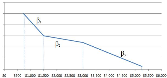
Rather than estimate a single slope (parameter) that characterizes a smooth relationship from $725 to $5,250, we are in this case fitting three slopes (β1, β2 and β3). The particular function above suggests that this respondent (remember that these betas are computed at the individual level) reacts more strongly to price changes between $725 and $1,500, and then less strongly to prices between $1,500 and $3,000. Then, the reaction is stronger again for prices higher than $3,000.
One could specify as many breakpoints as desired along the price continuum, but each additional breakpoint leads to another parameter to be estimated, and overfitting (including reversals) will eventually result. A key decision is where to place the breakpoints. It would be a mistake to place breakpoints such that very few products seen by respondents actually fell within a range bounded by two breakpoints. In the example above, if very few products were evaluated that fell in the range $750 to $1,500, the model would have very little information by which to obtain a stable estimate of β1. We recommend you run Analysis | Analysis Manager | Counts and look at the results on the Summed Price Frequencies tab of the resulting report. This allows you to view the distribution of prices of the product concepts shown to respondents to help you determine appropriate breakpoints.
The benefit of piecewise functions is that they will provide much better fit to the data than a linear function if the price function is truly non-linear. The drawbacks are that they lead to more parameters to estimate, and importantly that the analyst must determine the appropriate number and position of the breakpoints. We also restrict you from estimating interaction terms involving piecewise Price, as such designs are often deficient. Why is this so? Consider an interaction between brand and price, where some brands never occur in the high tier range. We'll be attempting to estimate betas for interaction effects where there is no information in the design matrix.
If the piecewise function is used, we simply carry the utility forward to the market simulator just for the prices corresponding to the end points and breakpoints for each respondent. When simulating prices between adjacent breakpoints, the market simulator applies linear interpolation. Thus, using the piecewise model results in utilities associated with discrete price levels (determined by the analysis) for use in the market simulator--the same process as is used in Sawtooth Software's ACA, CBC, and CVA systems. However, the choice of specific price levels is done post hoc rather than prior to fielding the study.
(Advanced Note: We temporarily transform whatever price range you provide to the range -x to +x, where x is the number of price parameters to estimate in the model so that HB converges more quickly. Then, we re-expand the parameters back to the original scale when reporting the final utilities.)
Recommendations:
When using piecewise functions for summed price, it may take significantly longer for HB to converge (than the default settings) and for the piecewise price parameters to oscillate across iterations with less certainty than other part-worth parameters in your study. Therefore, you may wish to increase the number of initial iterations (prior to assuming convergence) to something like 50K or more and also to increase the number of used iterations to 50K or more. As the number of cutpoints increases in your piecewise price specification, we especially encourage you to increase the number of initial and used iterations.
In general, we recommend piecewise function that use from 2 to 6 breakpoints (aside from the endpoints). Research at the 2013 Sawtooth Software Conference presented by the SKIM Group suggests that even more breakpoints (potentially a dozen or more) is potentially useful for ACBC studies, as long as you constrain price to be negative. This is based on only one study, so we would want to see additional evidence before recommending this generally.
We recommend you first run HB without utility constraints on the piecewise price function (with more initial and used iterations than the defaults) to check whether the utility for price generally decreases as price increases, as would be expected. If you confirm that price generally has a negative effect on utility over the entire price range, we recommend re-running HB and constraining the price function (negative slope).
Even though we restrict you from estimating interactions involving piecewise price, note that the very nature of creating a piecewise coding should inherently capture some interaction effects with price. For example, if premium brands are associated with a relatively large level-based price, then the beta associated with the upper price range will to a great extent be estimated specific to the occurrence of premium brands.